Showing posts with label Data analysis. Show all posts

Wednesday, October 7, 2020

Usage Of PROPER Function In Excel

Basically, Proper function is a built-in function in Excel which can be considered as a string or text conversion function like Upper & Lower function. Generally, it only capitalize the first letter of a word in a given text string and the return value will be considered as proper case.


N.B. If you are unsure about the process of UPPER & Lower function in Excel, then please check below URL’s first, which will give you a clear concept about the working principle of these sorts of functions.


URL: http://www.tutorialabc.com/2020/08/upper-function-in-excel.html

URL: http://www.tutorialabc.com/2020/09/lower-function-in-excel.html


Basic Syntax

=PROPER(text)


It passes a single argument, “text” – which text will be converted to proper case.


Notes: This function can be available from Excel 2000 to up-to-date version of Excel. And, Proper function will not consider - Spaces, numbers and punctuation marks.


Example:

Let’s consider, we have a sample set of data in the worksheet. 

(Working Data)


We will get the result, by using the PROPER function, ‘=PROPER(A1)’

Result: James Bond

And, ‘=PROPER(A2)’

Result: Hello! World


So, to get the exact result, please take a closer look on the below screenshots and follow along with the sequence. Hopefully, it will help you to understand the PROPER function in excel properly.


(PROPER function syntax)


(Proper Case)


(Conditions Unaffected)

For any query or suggestions, feel free to contact us and stay with tutorialabc.com for more Excel-based contents.


Tuesday, September 8, 2020

Usage Of LOWER Function In Excel

LOWER function in Excel works in a similar manner of UPPER function but it will do the opposite process of UPPER function. In brief, The LOWER function returns a lower case format of a given text. If you are unsure about the process of UPPER function then please check below URL first, which will give you a clear concept about the working principle of these sort of functions.


Basic Syntax
=LOWER(text)

It passes a single argument, “text” – which text will be converted to lower case.


Example


Suppose, you have a wide range of text in a spreadsheet which are in upper case or in some different format which give you a little bit disturbance to resolve your project with Excel. In that case, you may try to use the LOWER function to sort out the problem.


But, keep in mind that - Spaces, numbers and punctuation will be unaffected in LOWER function.

For the demonstration, we use some upper case text including space, number and punctuation markup and finally, we will get the lower case version of those text using LOWER function.

So, please take a closer look on the below screenshots and follow along with the sequence. Hopefully, it will help you to understand the LOWER function in excel properly.

(Working Data)


(LOWER function Syntax)


Soon, we will provide a similar type of tutorial known as PROPER function in Excel and till then keep learning and stay with tutorialabc.com! For any query or suggestions, feel free to contact

Friday, August 28, 2020

Usage of UPPER function in Excel


UPPER function in excel converts a given text into an upper case version. But, it will not affect on any numbers or punctuation marks at all. This function will help you to sort out a spreadsheet where most of the text entries are in lowercase. By using, UPPER function you can simply and very quickly resolve the issue.

Basic Syntax
=UPPER(text)

It passes a single argument, “text” – which text will be converted to upper case.

Example
Suppose, you have a wide range of text in a spreadsheet which are in lower case format and you want to convert those texts into upper case. Also, have a number value and punctuation and you want to use UPPER function to look at the differences.

“john”, “doe”, “9871”, “Hi!” are some values in a your spreadsheet. Now, follow the below image sequences and try it out by yourself. Hopefully, it will help you to understand the UPPER function in excel properly.

(Sample Data)

(Writing UPPER function)

(Selecting text from the cell)


(After converted to upper case)

(Ignoring numbers & punctuation)

Next, we will provide a tutorial on LOWER function in Excel and till then keep learning and stay with tutorialabc.com! For any query, feel free to contact us.


Tuesday, August 25, 2020

Working with ARABIC Function in MS-Excel


The Arabic function converts a Roman numeral into an Arabic numeral in Excel Spreadsheet. Basically this function works just the opposite of the ROMAN function of Excel. Check the ROMAN function tutorial here,


In simple words, Arabic function can convert Roman numerals into standard text format.

Syntax


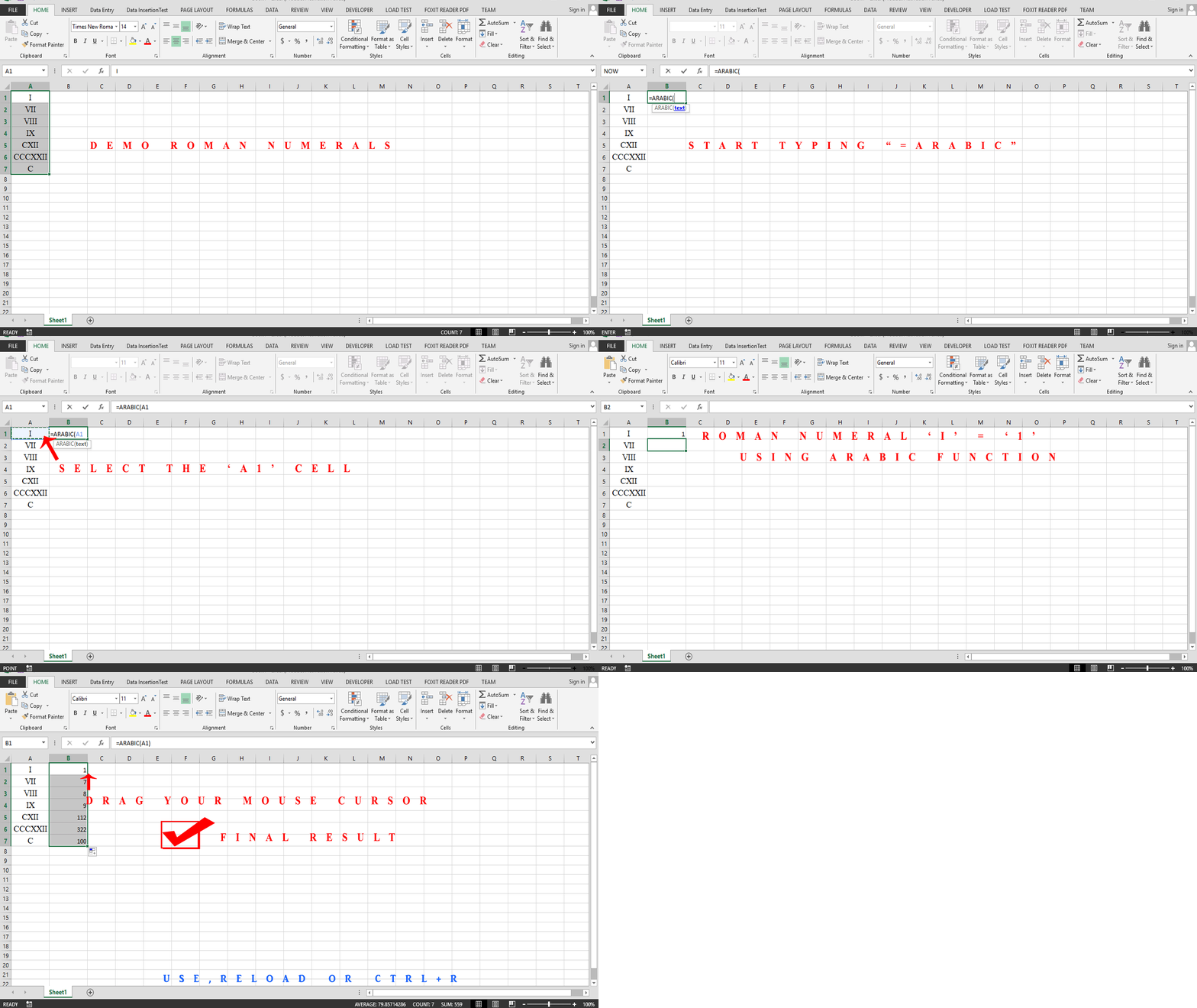
=ARABIC(text)


Here, the text argument is a text representation of a Roman numeral and it supports maximum 255 characters.

Keep in mind,

If the text argument passed directly to the function, use Double-Quotes, else you will get #NAME? Error.

Example

=ARABIC(“XI”) , correct

=ARABIC(XI), incorrect and produce #NAME? Error.

If an empty text string is passes as an argument, the Arabic function returns the value 0. Excel’s earlier version before 2013, Arabic function wasn’t available.

Here, we are adding a GIF file which converts some ROMAN numerals into regular numbers by using the ARABIC function. Please take a close look at the GIF and reload the GIF or Press Ctrl+R on your browser to watch the GIF repeatedly.


That’s set! ARABIC function is a very tiny piece of built-in function in Excel, but with the help of this function you may save your precious time. So, if anything remains unclear to you or have any query, feel free to contact us. Thank you and stay with tutorialabc.com for more interesting Excel-based tutorials. 


Sunday, June 28, 2020

How simply Age can be calculated in Excel


Well, sometimes it is necessary to extract the correct age of a person from a dataset in an excel file and with a simple trick or can say, by using a formula in Excel, you can calculate the age of any person based on the data provided to you.

The math behind the age calculation or how old you are based on some criteria. Basically, it requires the Date of Birth (DOB) and the current date. And, the current date can be obtained by using Today () function which is a built-in function of Excel. Then just need to find the difference from the result of Today () to DOB and divide the entire value by 365 as you know 365 is the equivalent of a year.

One thing to remember here, the number format of the excel sheet has to be in General format to get the desired result. Please check the number format of your excel sheet before proceeding.

General formula:

=(Today () - DOB)/365


Though by using this general formula you will get the correct age of a person but it will provide you some fractional value after the year. To remove the fractional part you need to use ‘int’ before the general formula. Like,

      =int(Today () - DOB)/365

Now, you will get the exact year of that person based on the Date of birth till today.

Here, we are adding some screenshots with very few data and steps to perform the above-mentioned calculation. Please look carefully and follow along with those steps. Hopefully, you’ll understand it clearly.


If you have slight confusion about anything or have any queries, please feel free to knock us via our contact page. Thanks for staying with tutorialabc.com!


Friday, June 5, 2020

Working With Rank Function in Excel

Rank function is a very useful function in case of ranking numeric values within a list. It will return rank of a number against a range of numbers and will ignore other sorts of values including text, character etc.

In this short tutorial, we’ll learn how you can use rank function and what sort of result you will get by using this function. Hopefully, this beginner-level tutorial will give you a clear understanding of rank function and you will be able to work with it independently.

Let’s start,

Basic Syntax
= RANK(number, ref, [order])

As you can see from the syntax, Rank function passes three arguments which are number, ref & order.
  • number: number is the first argument of rank function and it means the number we would like to check within a list of numbers.
  • ref: this argument is used to compare within the list of numbers. We could select the entire cell by referencing the cell or we could also select some values within the cell manually.
  • order: this argument is optional but it’ll help you to maintain the order of the list and rank them according to descending or ascending order.

-         0 or leave the argument empty: It will rank the list in default descending order.
-         1 : for ascending order please type 1 in the last argument field of the rank function.

Example
Suppose, you have a worksheet which contains data like the below screenshot and from those data you want to rank them based on Total Profit


So, now at first, choose the blank cell E2 and start typing “=Rank” and click on the suggested Rank function, like in the below image,


Then just pass the arguments according to the format of the function and every argument will be separated by a comma.


For our case, we just select the D2 cell as the first argument of the rank function, then select all other cells of the Total Profit header which contains numeric values as reference (the second argument) and at last, choose descending order so we select ‘0’ as rank functions final argument.


And, we get the rank for that number within the list.


Finally, just drag your mouse to the last value of the worksheet


and you will get the ranks of those numeric values within the list. Like the below screenshot,


Finally, we are adding a GIF image for you so that you can cope with the total process of the Rank function.


Isn’t it simple! Just try to choose the other ways of passing the arguments on your own and see the difference. It will help you to understand the Rank function more precisely. Thanks for staying with tutorialabc.com!

If you have any queries, please let us know through our contact page. 

Thursday, April 23, 2020

Usage of SUMIF & SUMIFS in Excel

Today we will cover two basic yet very essential functions of MS Excel.
  1. SUMIF &
  2. SUMIFS

We believe, you already know the functionality of sum function. If you don’t know, please check out this SUM function tutorial.

SUMIF and SUMIFS have the same functionality likewise a SUM function but these two functions contain additional criteria to lookup the entire data table and based on those criteria it performs the sum operation.

Keep in mind, SUMIF function accepts only one criteria whereas SUMIFS function takes multiple criteria.


Introduction of SUMIF

SUMIF comes up with a comparison operator like greater than, less than or equal, etc, It supports both character and integer.

When there are a large number of data set their manual calculation is ineffective when you have to find out the range of sum based on condition. 

General syntax


=SUMIF (range, criteria, [sum_range])


Example & Working way,

Just think of a biscuit company inventory, where you need to find out how many kgs of flour ingredients is available there. So you must need a condition to apply in the sum that only flour ingredients need to sum up. Therefore, SUMIF function you can infuse a condition on SUM.

Now, for clear understanding, follow the below steps carefully.

1. Try to create or just copy & paste the below dataset on your excel worksheet as an example.

Product
Region
salesRep
Customer
Sales
bellen
South
zubbar
e
123
sun
East
zubbar
a
234
bellen
west
zubbar
g
345
sun
north
zubbar
w
456
zasa
East
zubbar
e
567
bellen
west
zubbar
e
678
zisa
north
zubbar
a
789
bellen
west
zubbar
g
344
sun
north
zubbar
w
1222
mss
East
akib
e
2100
zasa
west
akib
e
2978
bellen
East
akib
a
3856
sun
west
akib
g
4734

2. Then choose a blank cell and type “=SUMIF (A2:A14,"bellen", E1:E14)” to calculate the sum of bellen product sales and you will get a result of 4568 Sales based on the criteria.

Then, try to work with other products from the dataset to calculate the sum of the sales of those products. Hopefully, it will give you a clear concept, how actually SUMIF function work in MS-Excel.

Introduction of SUMIFS

SUMIFS function is almost the same as SUMIF. It has the power where you can set multiple conditions or on excel sense criteria.

General syntax


=SUMIFS (sum_range, range1, criteria1, [range2], [criteria2], ...)


Example & Working way,

1. Again, copy & paste the given dataset on your excel worksheet or prepare one by yourself.

Product
Region
salesRep
Customer
Sales
bellen
South
zubbar
e
123
sun
East
zubbar
a
234
bellen
west
zubbar
g
345
sun
north
zubbar
w
456
zasa
East
zubbar
e
567
bellen
west
zubbar
e
678
zisa
north
zubbar
a
789
bellen
west
zubbar
g
344
sun
north
zubbar
w
1222
mss
East
akib
e
2100
zasa
west
akib
e
2978
bellen
East
akib
a
3856
sun
west
akib
g
4734


2. Choose a blank cell where you want to show your sum result and start typing “=SUMIFS(E2:E14,A2:A14,"bellen",C2:C14,"zubbar")” to calculate the total sales of the product bellen which is sold under a salesRep named zubbar. You will get a result of 1490 Sales based on those criteria.

Hopefully, this tutorial makes some sense and got a clear understanding, how actually SUMIF & SUMIFS function work and also know the difference between them.

That’s set for today. If you have any inquiries or suggestions regarding this please write to us in the comment section. Stay with tutorialabc for more easy excel tutorials.